7 ARIMA Models

The ARMA models of Chapter 5 require a stationary series, which is why we fit them to returns, not prices. The ARIMA model removes that restriction. The “I” stands for integrated: an ARIMA model first differences the series enough times to make it stationary, then fits an ARMA to the result. This is the bridge between the non-stationarity of Chapter 6 and the ARMA machinery of Chapter 5 — and, for our objective, it is what lets us model and forecast the price level itself, not just its returns.

There is an equivalence at the heart of this chapter that makes it short: because a log price is \(I(1)\) and its first difference is the log return, fitting an ARIMA(\(p,1,q\)) to the log price is exactly the same as fitting an ARMA(\(p,q\)) to the log return. Everything we learned in Chapters 3–5 therefore transfers directly; what is genuinely new is the price-level forecast.

7.1 Simple ARIMA models

An ARIMA model differences a non-stationary series \(d\) times to make it stationary, then fits an ARMA to the result — the “I” stands for integrated.

Write \(B\) for the backshift operator (\(B y_t = y_{t-1}\)) and \(\nabla = 1 - B\) for the first-difference operator, so \(\nabla y_t = y_t - y_{t-1}\). A series \(y_t\) follows an ARIMA(\(p,d,q\)) model if its \(d\)-th difference, \(w_t = \nabla^d y_t\), is a stationary ARMA(\(p,q\)):

\[ \underbrace{\phi(B)}_{\text{AR}(p)}\, \underbrace{(1-B)^d}_{\text{difference } d\text{ times}}\, y_t = \phi_0 + \underbrace{\theta(B)}_{\text{MA}(q)}\, a_t, \tag{7.1}\]

where \(\phi(B) = 1 - \phi_1 B - \cdots - \phi_p B^p\) and \(\theta(B) = 1 + \theta_1 B + \cdots + \theta_q B^q\). In words: difference \(d\) times to reach stationarity, then model what remains as ARMA(\(p,q\)). The three orders are the AR order \(p\), the degree of differencing \(d\), and the MA order \(q\).

For our data \(d = 1\): a log price is \(I(1)\) (Chapter 6), so one difference — the log return — is stationary. Thus ARIMA(\(p,1,q\)) on the log price = ARMA(\(p,q\)) on the log return, and the special cases we already met reappear with new names:

ARIMA(0,1,0) — \(\nabla y_t = a_t\) — is the random walk.
ARIMA(0,1,0) with a constant is the random walk with drift, the log-price model of Section 6.3.

7.2 Properties of ARIMA models

Two of the three orders are chosen by machinery we have already built, and the third property is what makes ARIMA forecasts distinctive.

The differencing order \(d\) is a unit-root question. You do not read \(d\) off the ACF; you determine it with the ADF and KPSS tests of Chapter 6. If the level is \(I(1)\), take \(d=1\); if the difference were still non-stationary you would take \(d=2\), and so on. Over-differencing is a real cost (it injects a non-invertible MA unit root), so we difference the minimum number of times — for our log prices, once.

Once differenced, it is just ARMA. The stationary series \(w_t = \nabla^d y_t\) obeys all the ARMA properties of Chapter 5: stationarity via the AR roots, invertibility via the MA roots, ACF/PACF identification of \(p\) and \(q\).

Forecasts of an integrated series fan out. This is the property that sets ARIMA apart. Because differencing was needed, the level \(y_t\) carries a unit root, and the variance of its \(h\)-step forecast grows without bound with the horizon — for the random walk with drift, \(\operatorname{Var}[\hat y_T(h)] = h\sigma^2\), so the forecast interval widens like \(\sqrt{h}\). The point forecast is a straight line at the drift slope; the interval around it is a widening cone. Contrast this with the return forecasts of Chapters 3–5, whose intervals were essentially flat: the return is stationary, so its uncertainty does not accumulate, but the price is its running sum, so uncertainty piles up.

7.3 Identifying ARIMA models

Identification is a clean three-step recipe that reuses everything so far:

Choose \(d\) with unit-root tests (Chapter 6). Our log prices are \(I(1)\) \(\Rightarrow d = 1\).
Difference the series \(d\) times. Here \(\nabla(\log \text{price}) = \log \text{return}\).
Identify \(p\) and \(q\) on the differenced series using the ACF/PACF, EACF, or an information criterion (Section 3.5.2, Section 4.3, Section 5.3).

Step 3 is work we have already done — the ARMA orders of the returns are the \((p,q)\) of the log-price ARIMA. In practice auto.arima performs all three steps automatically, running the unit-root test for \(d\) and a stepwise BIC search for \(p,q\).

R
Python

library(forecast)
logprice <- function(sym) {
  d <- read.csv(sprintf("data/%s.csv", sym)); d$Date <- as.Date(d$Date)
  log(d$Adjusted[d$Date <= as.Date("2026-07-01")])
}
# auto.arima picks d (via unit-root tests) and p,q (via BIC) on the log PRICE
for (s in c("AAPL","MSFT","AMZN","SPX","GLD","GCF"))
  cat(s, ":", forecast::arimaorder(auto.arima(logprice(s), ic = "bic")), "\n")

# equivalently, ARIMA(1,1,1) on the log price == ARMA(1,1) on the return:
Arima(logprice("SPX"), order = c(1, 1, 1), include.drift = TRUE)

import pandas as pd, numpy as np
from statsmodels.tsa.arima.model import ARIMA

def logprice(sym):
    d = pd.read_csv(f"data/{sym}.csv", parse_dates=["Date"]).set_index("Date")
    return np.log(d[d.index <= "2026-07-01"]["Adjusted"])

# ARIMA(1,1,1) with drift on the log price  ==  ARMA(1,1) on the return
fit = ARIMA(logprice("SPX"), order=(1, 1, 1), trend="t").fit()
print(fit.summary())

The log-price ARIMA orders are just the return ARMA orders from Table 5.2 with \(d=1\) inserted:

Table 7.1: ARIMA models for the log prices

Ticker	\(d\) (unit-root tests)	ARMA order on returns	ARIMA on log price
AAPL	1	(0,0)	ARIMA(0,1,0) + drift
MSFT	1	(0,1)	ARIMA(0,1,1) + drift
AMZN	1	(0,0)	ARIMA(0,1,0) + drift
SPX	1	(1,1)	ARIMA(1,1,1) + drift
GLD	1	(0,0)	ARIMA(0,1,0) + drift
GCF	1	(0,0)	ARIMA(0,1,0) + drift

Table 7.1 carries a sharp message. For four of the six series the best model for the log price is ARIMA(0,1,0) with drift — the random walk with drift. That is not a modelling failure; it is the formal statement that these prices are unforecastable beyond their average drift, so the naive “tomorrow’s price = today’s price + average daily move” is the best you can do. Only Microsoft (a lone MA term) and the S&P (the ARMA(1,1) structure of Chapter 5) add anything, and — as we saw — what they add is worth well under \(2\%\) of return variance. Fitting the S&P’s ARIMA(1,1,1) recovers exactly the \(\hat\phi_1 = -0.475\), \(\hat\theta_1 = +0.355\) we estimated on the returns; the “I” simply lets us state the model, and forecast, in the units of the price.

7.4 Goodness of fit

Because ARIMA(\(p,1,q\)) on the log price is ARMA(\(p,q\)) on the return, the fit diagnostics are identical to Section 5.4: the residuals should be white noise (Ljung–Box on \(\hat a_t\)), and the model explains the same tiny fraction of return variance (\(R^2 \approx 0.018\) for the S&P). The one thing that changes is what a “good fit” buys you — a coherent model of the price, with the correct unit-root-driven uncertainty, rather than of the return alone. And, as in every chapter, the squared residuals remain autocorrelated: ARIMA has captured all the linear structure there is, and the volatility clustering is still untouched.

7.5 Forecasting the price level

Here is what ARIMA adds that ARMA-on-returns could not: a forecast of the price, with an honestly widening interval. For the random-walk-with-drift case the forecast is simply

\[ \hat y_T(h) = y_T + h\,\mu, \qquad \operatorname{Var}[\hat y_T(h)] = h\,\sigma^2, \tag{7.2}\]

where \(y_T\) is the last log price, \(\mu\) the drift (mean log return), and \(\sigma^2\) the return variance. The point forecast is a straight line rising at the drift rate; the \(95\%\) interval, \(\hat y_T(h) \pm 1.96\,\sigma\sqrt{h}\), widens as \(\sqrt{h}\). Exponentiating gives the price and its (asymmetric, lognormal) band. The carousel below shows this for all six tickers over — and beyond — the July holdout.

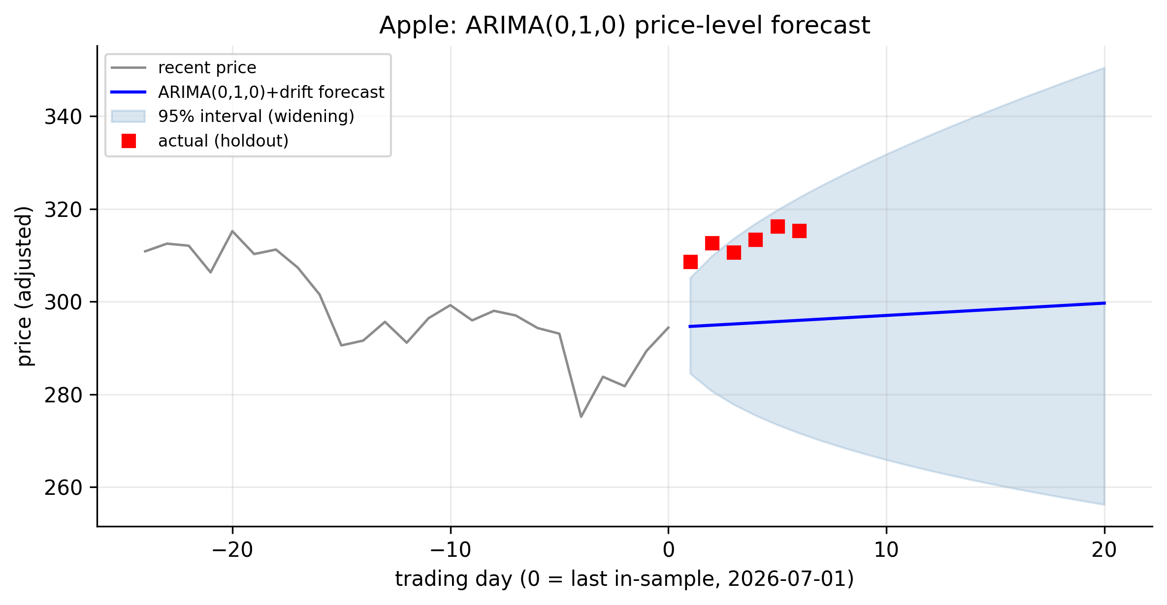
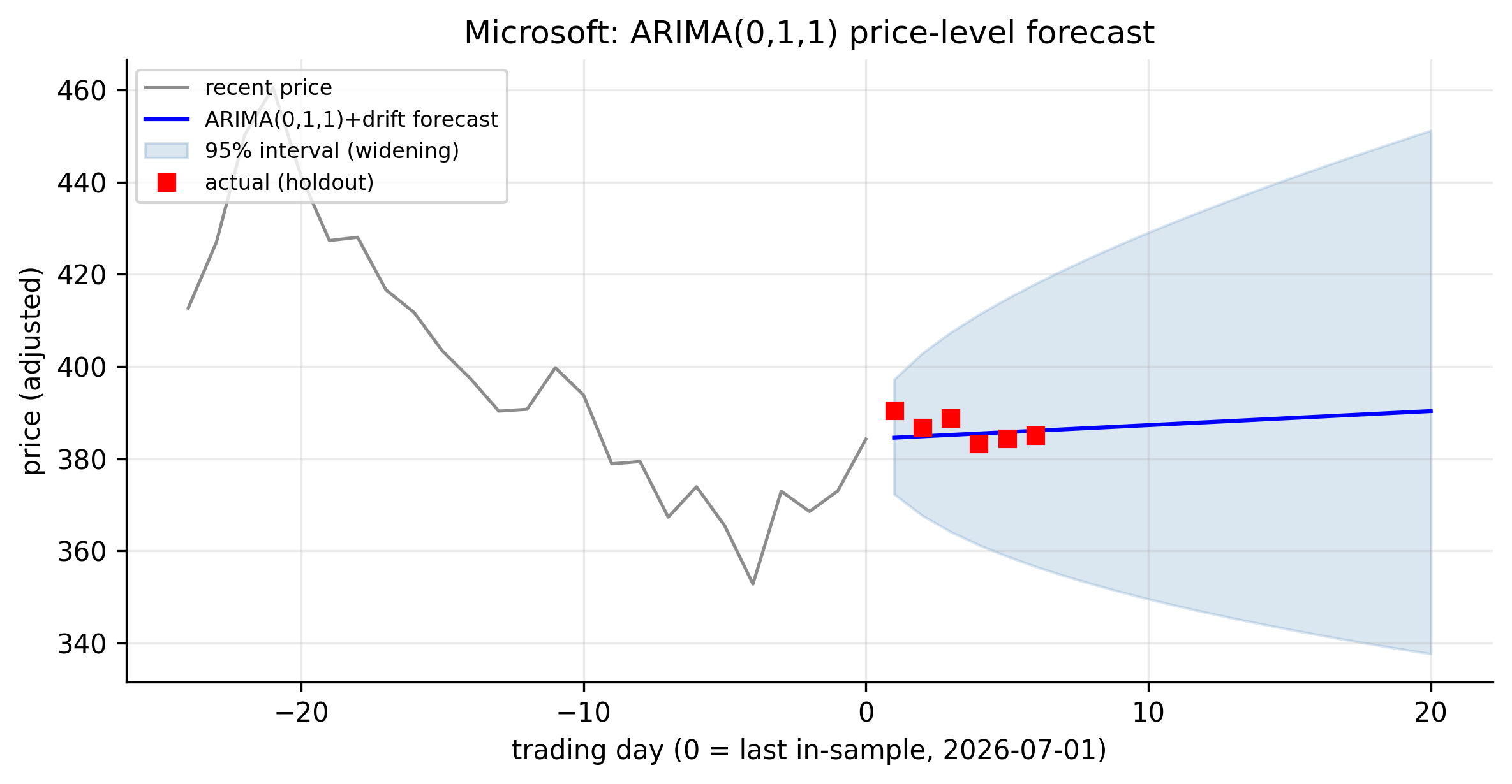
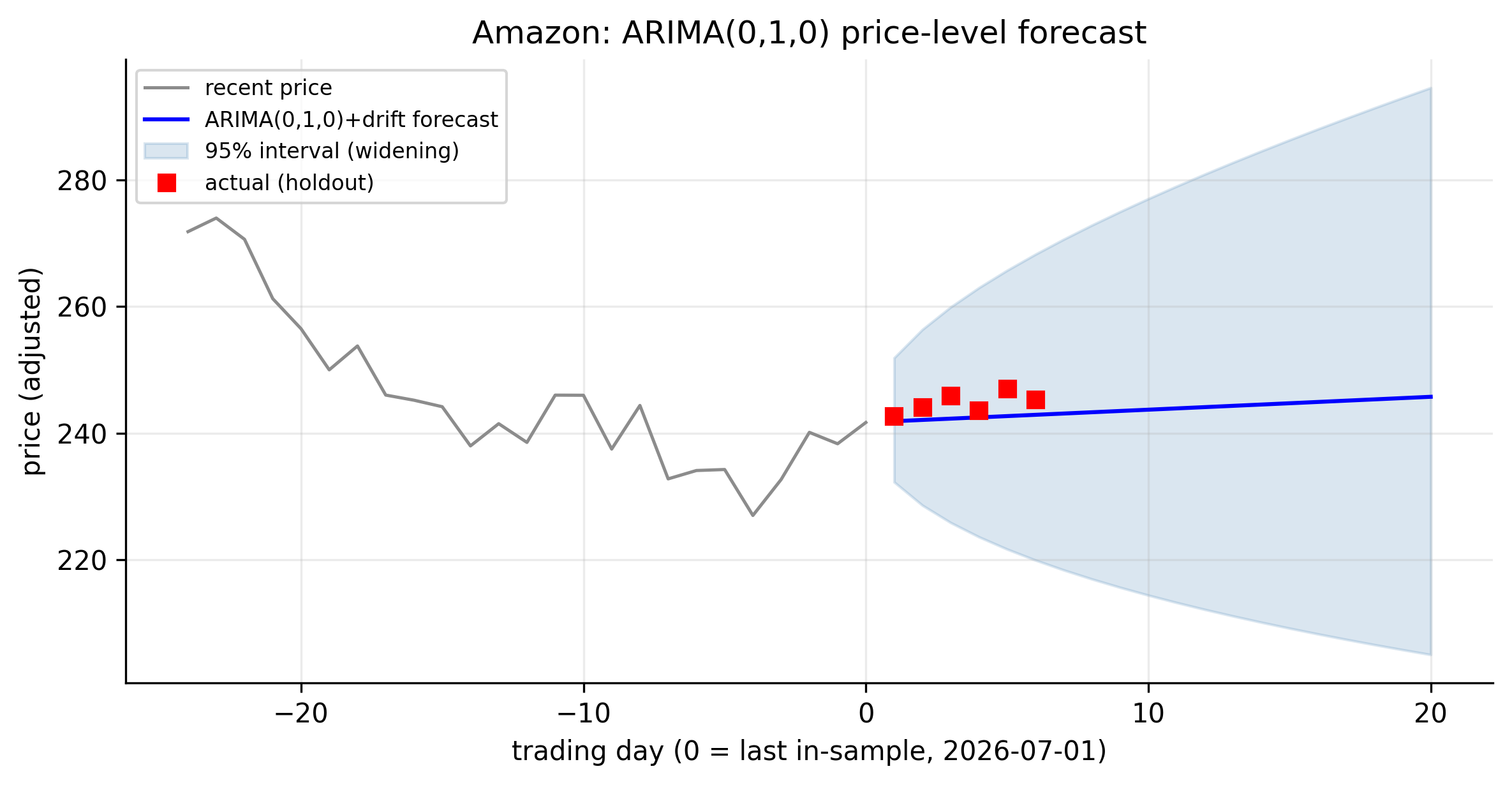
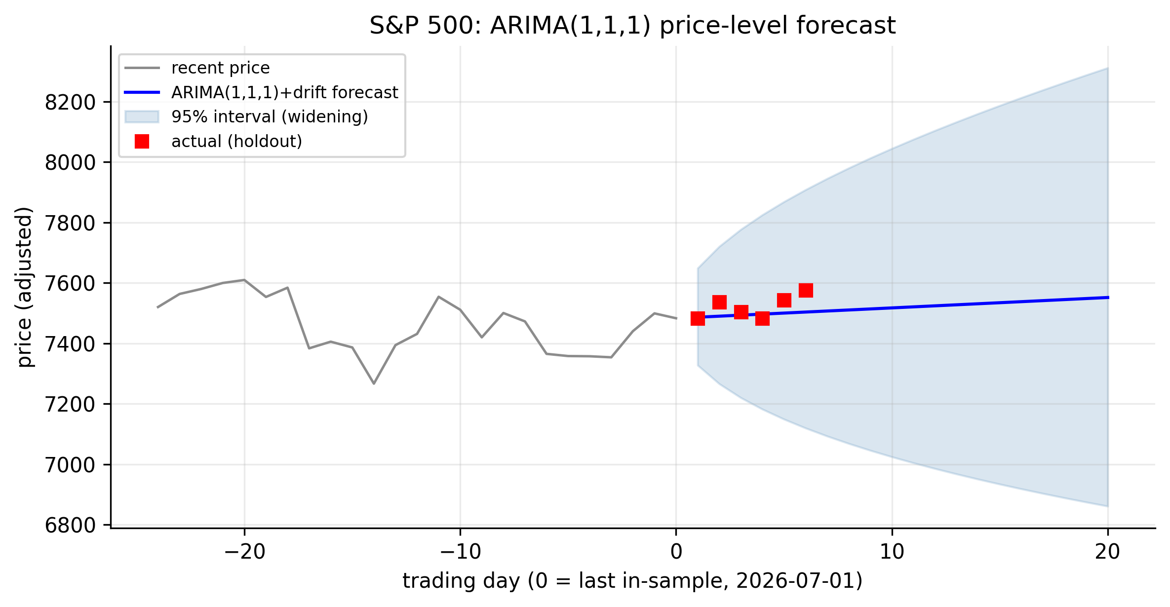
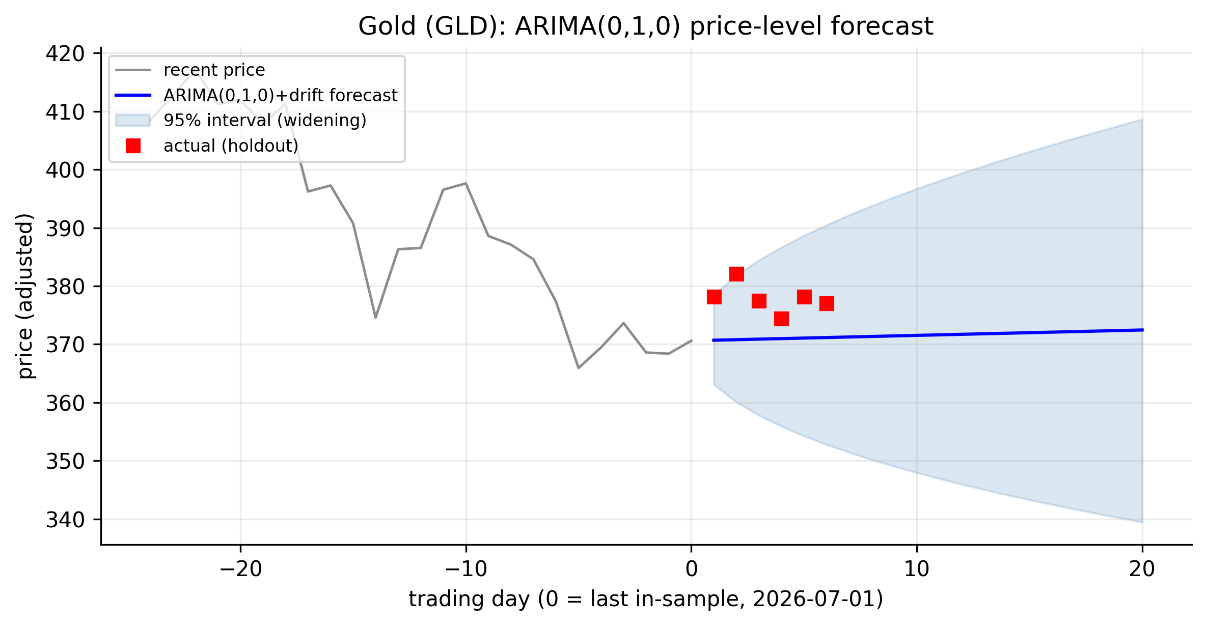
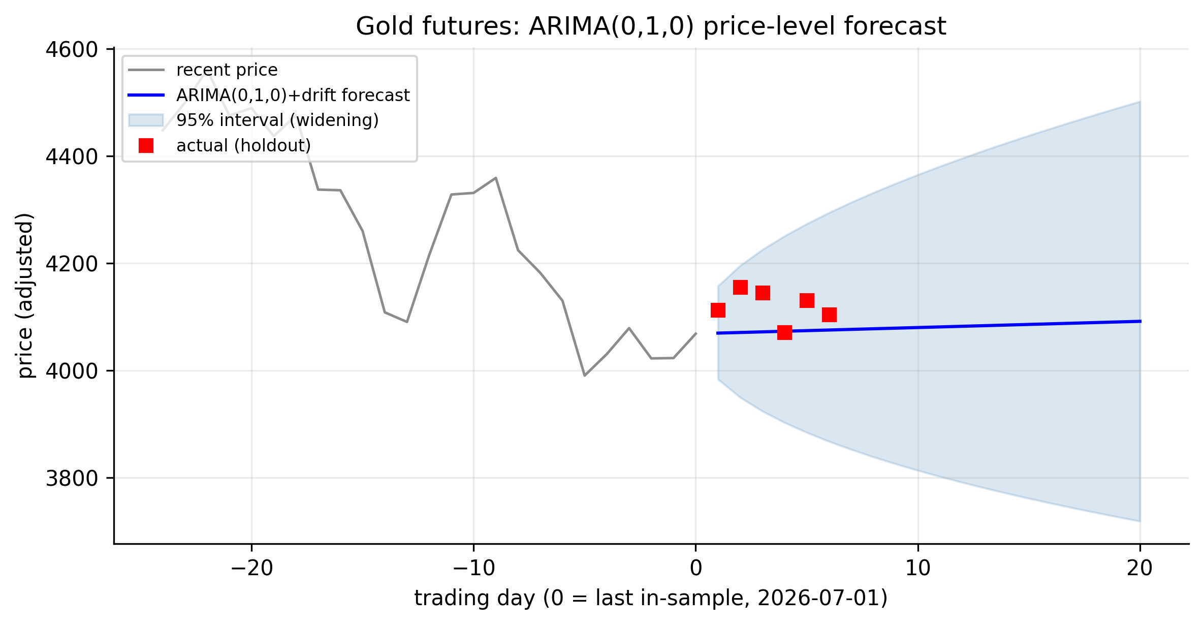
Gold futures ARIMA(0,1,0) price forecast

Every panel has the same anatomy: a nearly straight forecast line rising at the series’ drift, wrapped in a cone that widens with the horizon, with the realised holdout prices scattered inside it. The cone is the honest part. Ten trading days out, the S&P’s \(95\%\) price interval already spans roughly \(\pm 3\%\); twenty days out, more. This is the unit root made visible: uncertainty about the price compounds with time even though uncertainty about each day’s return does not. It is also the practical limit of linear forecasting for these series — the point forecast is only ever the drift line, and the value the model provides is a correctly-sized measure of how wrong that line could be.

7.6 Concept check

Decide first, then expand each answer.

Q1. In ARIMA(\(p,d,q\)), what does the middle term \(d\) do?

(a) Sets the number of AR lags.
(b) Specifies how many times the series is differenced to make it stationary.
(c) Sets the number of MA lags.
(d) Is the forecast horizon.

Show answer

(b). \(d\) is the degree of differencing — the “I” for integrated. Difference \(d\) times to reach stationarity, then fit ARMA(\(p,q\)) to the result.

Q2. An ARIMA(0,1,0) model is:

(a) white noise.
(b) a random walk (a random walk with drift if a constant is included).
(c) an AR(1).
(d) always non-invertible.

Show answer

(b). \((1-B)y_t = a_t\) is the random walk; adding a constant gives the random walk with drift — the log-price benchmark of Section 6.3.

Q3. Fitting an ARIMA(1,1,1) to the log price is equivalent to fitting what to the log return?

(a) an ARIMA(1,1,1).
(b) an ARMA(1,1).
(c) an AR(1).
(d) nothing — they are unrelated.

Show answer

(b). The first difference of the log price is the log return, so ARIMA(\(p,1,q\)) on the price equals ARMA(\(p,q\)) on the return. Our S&P fit recovers the same \(\phi_1=-0.475\), \(\theta_1=+0.355\).

Q4. Why does an ARIMA price-forecast interval widen with the horizon while the return-forecast interval stays roughly flat?

(a) A plotting artifact.
(b) The price carries a unit root, so forecast variance accumulates (\(\approx h\sigma^2\)); the return is stationary, so its variance does not.
(c) The drift grows over time.
(d) The model is misspecified.

Show answer

(b). The price is the running sum of returns; uncertainty compounds, giving a \(\sqrt{h}\)-widening cone. Stationary returns have bounded, non-accumulating variance.

Q5. How is the differencing order \(d\) determined?

(a) From the PACF cutoff.
(b) From unit-root tests (ADF/KPSS) — you difference until the series is stationary.
(c) It is always 1.
(d) By maximising \(R^2\).

Show answer

(b). \(d\) is a stationarity question, settled by the unit-root tests of Chapter 6 (here \(d=1\)), not by the ACF/PACF, which identify \(p\) and \(q\) on the already-differenced series.

Key takeaways

ARIMA(\(p,d,q\)) (Equation 7.1) differences a series \(d\) times to reach stationarity, then fits ARMA(\(p,q\)); the “I” is for integrated.
For our data \(d=1\), so ARIMA(\(p,1,q\)) on the log price = ARMA(\(p,q\)) on the log return — the Chapters 3–5 results transfer unchanged.
Identify in three steps: choose \(d\) by unit-root tests, difference, then identify \(p,q\) as before (auto.arima automates all three).
Four of our six log prices are ARIMA(0,1,0) + drift — a random walk with drift; only Microsoft and the S&P add (tiny) structure (Table 7.1).
ARIMA’s distinctive gift is the price-level forecast: a drift line inside a cone that widens like \(\sqrt{h}\) — the unit root made visible, and the honest limit of linear forecasting for these series.