5 ARMA Models
The AR model built the mean from past values; the MA model built it from past shocks. The ARMA model uses both. For most of our series this changes nothing — they are white noise, and no combination of terms helps. But for the one series with genuinely richer structure, the S&P 500, ARMA delivers the payoff the previous two chapters kept pointing toward: it captures with two parameters what the pure AR model needed eight to describe. That is the whole case for ARMA — parsimony.
We follow the same path a final time: definition, properties, identification, goodness of fit, forecasting, across the six tickers.
5.1 Simple ARMA models
An ARMA model combines an autoregressive part (past values) and a moving-average part (past shocks) in a single model.
An ARMA(\(p,q\)) model combines an order-\(p\) autoregression with an order-\(q\) moving average:
\[ r_t = \phi_0 + \sum_{i=1}^{p}\phi_i\, r_{t-i} + a_t + \sum_{j=1}^{q}\theta_j\, a_{t-j}, \tag{5.1}\]
with \(\{a_t\}\) white noise. The AR part links today’s return to recent returns; the MA part links it to recent shocks. AR(\(p\)) is the special case \(q=0\), MA(\(q\)) is \(p=0\), and white noise is ARMA(\(0,0\)). The ARMA(1,1) — one of each — is the smallest genuinely mixed model and the one our data will actually use: \(r_t = \phi_0 + \phi_1 r_{t-1} + a_t + \theta_1 a_{t-1}\).
5.2 Properties of ARMA models
ARMA inherits one condition from each parent. It is stationary when the roots of the AR polynomial \(1 - \phi_1 z - \cdots - \phi_p z^p\) lie outside the unit circle (the AR condition), and invertible when the roots of the MA polynomial \(1 + \theta_1 z + \cdots + \theta_q z^q\) do (the MA condition). When stationary, its mean is \(\mu = \phi_0/(1 - \phi_1 - \cdots - \phi_p)\), exactly as in the AR case.
The property that matters most for practice concerns identification. In a mixed model, both the ACF and the PACF tail off — neither cuts off cleanly:
| Process | ACF | PACF |
|---|---|---|
| AR(\(p\)) | tails off | cuts off after \(p\) |
| MA(\(q\)) | cuts off after \(q\) | tails off |
| ARMA(\(p,q\)) | tails off | tails off |
This is inconvenient: the clean order-reading trick that worked for pure AR and MA fails for ARMA, because there is no cutoff to count. We need other tools, which is the subject of the next section.
One caution belongs here too — parameter redundancy. If an ARMA(1,1) has \(\phi_1 \approx -\theta_1\), the AR and MA factors nearly cancel (a “common factor”), leaving a model that is effectively white noise but described by two large, unstable, offsetting coefficients. Over-fitting ARMA invites exactly this pathology, which is why parsimony — and a criterion like BIC that enforces it — is essential.
5.3 Identifying ARMA models
Because Table 5.1 offers no cutoff, ARMA identification uses different tools. Tsay’s preferred device is the Extended Autocorrelation Function (EACF), a table of significance markers whose triangular pattern of zeros has its top-left corner at the true \((p,q)\). In practice — and here — it is at least as common to search a grid of \((p,q)\) orders and let an information criterion choose, exactly as we did for the pure models but now over a two-dimensional grid. We fit every ARMA(\(p,q\)) for \(p,q \in \{0,1,2\}\) and pick the smallest BIC.
est_return <- function(sym) {
  d <- read.csv(sprintf("data/%s.csv", sym)); d$Date <- as.Date(d$Date)
  diff(log(d$Adjusted[d$Date <= as.Date("2026-07-01")]))
}
# grid search over (p, q); BIC selects
for (p in 0:2) for (q in 0:2) {
  f <- arima(est_return("SPX"), order = c(p, 0, q), method = "ML")
  cat(sprintf("ARMA(%d,%d)  BIC = %.1f\n", p, q, BIC(f)))
}
# Tsay's EACF is the alternative order-identification tool:
# TSA::eacf(est_return("SPX"))
import pandas as pd, numpy as np, itertools
from statsmodels.tsa.arima.model import ARIMA
def est_return(sym):
d = pd.read_csv(f"data/{sym}.csv", parse_dates=["Date"]).set_index("Date")
return np.log(d[d.index <= "2026-07-01"]["Adjusted"]).diff().dropna()
for p, q in itertools.product(range(3), range(3)):
bic = ARIMA(est_return("SPX"), order=(p, 0, q)).fit().bic
print(f"ARMA({p},{q}) BIC = {bic:.1f}")The BIC over the low-order grid (shown as a difference from each series’ best, \(\Delta\text{BIC}\), so the selected model is at \(0.00\)):
| Ticker | ARMA(0,0) | ARMA(1,0) | ARMA(0,1) | ARMA(1,1) | Selected |
|---|---|---|---|---|---|
| AAPL | 0.00 | 2.85 | 2.96 | 10.05 | white noise |
| MSFT | 27.84 | 0.59 | 0.00 | 8.09 | single lag (MA/AR 1) |
| AMZN | 0.00 | 7.31 | 7.30 | 11.95 | white noise |
| SPX | 52.42 | 6.71 | 13.42 | 0.00 | ARMA(1,1) |
| GLD | 0.00 | 8.20 | 8.19 | 15.37 | white noise |
| GCF | 0.00 | 4.47 | 4.37 | 12.34 | white noise |
Table 5.2 closes the arc of the last three chapters. Four series — Apple, Amazon, and both gold contracts — are white noise: ARMA(0,0) wins, and every added AR or MA term only raises BIC. Microsoft’s lone lag-1 correlation is captured equally by ARMA(1,0) or ARMA(0,1) — the AR(1)≈MA(1) equivalence from Section 4.3.1 — and the mixed ARMA(1,1) is a wasted parameter (BIC worse by \(8\)). The exception, once again, is the S&P 500: here ARMA(1,1) is the clear winner, beating white noise by \(52\) BIC points, the pure AR(1) by \(6.7\), and the pure MA(1) by \(13.4\).
Why does the mix succeed where neither pure model did? The S&P’s ACF changes sign — negative at lag 1 (\(-0.119\)), positive at lag 2 (\(+0.082\)) — an oscillating pattern that a single AR or MA term cannot produce but an ARMA(1,1) with \(\hat\phi_1 = -0.475\) and \(\hat\theta_1 = +0.355\) reproduces naturally (the negative \(\phi_1\) drives the alternation). Crucially, this ARMA(1,1) achieves the same fit as the AR(8) that BIC chose back in Table 3.4 — its \(R^2\) is about the same \(0.018\) — but with two parameters instead of eight. That is parsimony in action, and it is the reason ARMA exists.
\(\hat\phi_1 = -0.475\) and \(\hat\theta_1 = +0.355\) are much larger than the \(\approx -0.11\) we saw fitting pure AR(1)/MA(1). They are not redundant — \(\phi_1 \neq -\theta_1\), so the factors do not cancel — and together they imply exactly the small \(\rho_1 = -0.12\) and sign-flipped \(\rho_2 = +0.06\) we observe. Large offsetting coefficients that do nearly cancel would be the redundancy warning of Section 5.2; these do not.
5.4 Goodness of fit
The fitted S&P ARMA(1,1) passes the diagnostic that matters: its residuals are white noise (Ljung–Box on \(\hat a_t\) no longer rejects — the oscillating structure has been absorbed), and it does so with a residual standard deviation of \(1.0835\%\), essentially the AR(8) value. But the familiar ceiling still holds: an \(R^2\) of \(1.8\%\) means the model explains under one-fiftieth of the variance of daily S&P returns, and — as in every chapter so far — the squared residuals remain strongly autocorrelated (Figure 3.3). ARMA has wrung out the last of the linear mean structure; the volatility clustering is entirely untouched.
fit <- arima(est_return("SPX"), order = c(1, 0, 1))       # ARMA(1,1)
fit                                                        # coefficients & SE
Box.test(residuals(fit), lag = 10, type = "Ljung-Box")    # residuals white noise?
1 - fit$sigma2 / var(est_return("SPX"))                   # approx R^2
from statsmodels.stats.diagnostic import acorr_ljungbox
fit = ARIMA(est_return("SPX"), order=(1, 0, 1)).fit()
print(fit.summary())
print(acorr_ljungbox(fit.resid, lags=[10]))
print(1 - fit.resid.var() / est_return("SPX").var())5.5 Forecasting
The ARMA forecast blends the two behaviours we have already seen. The MA part contributes only for the first \(q\) steps (its finite memory of past shocks), after which the forecast follows the AR part’s geometric decay toward the mean. For an ARMA(1,1):
\[ \hat r_t(1) = \phi_0 + \phi_1 r_t + \theta_1 a_t, \qquad \hat r_t(h) = \phi_0 + \phi_1\, \hat r_t(h-1) \;\; (h \ge 2), \tag{5.2}\]
so the last shock \(a_t\) enters the one-step forecast, and from step two on it is pure AR(1) reversion. The carousel below runs the selected ARMA forecast for each ticker over the July holdout.
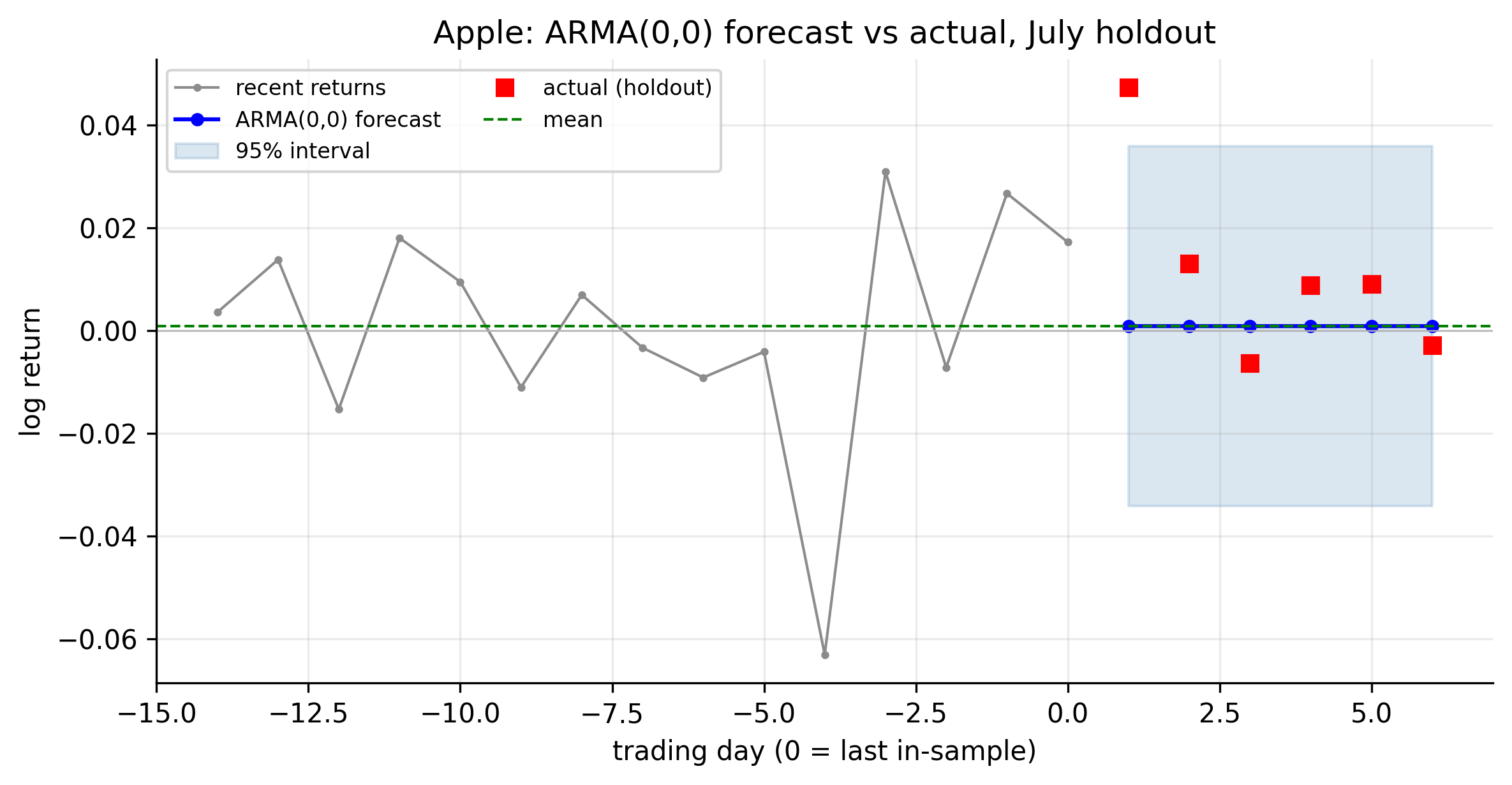
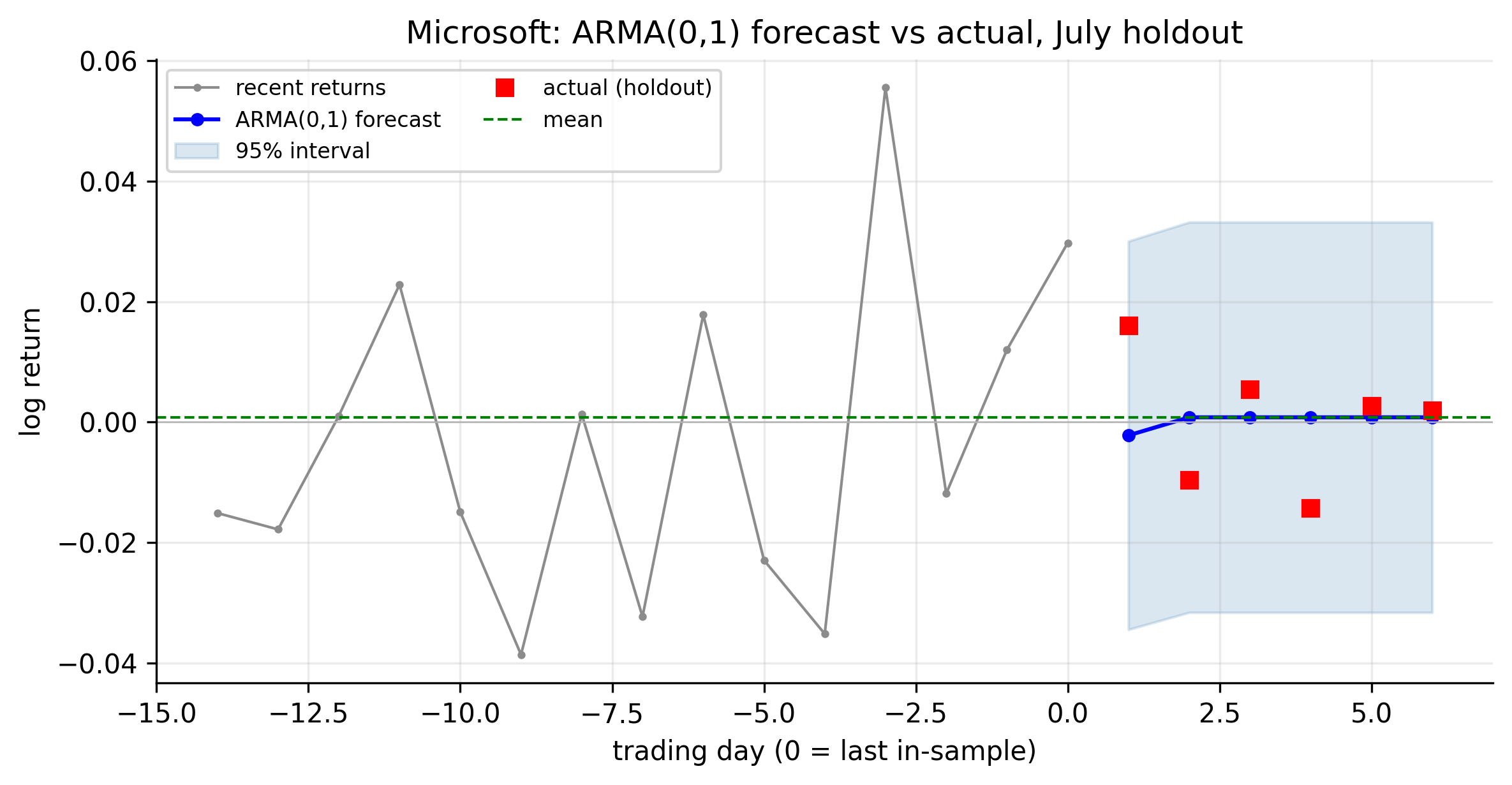
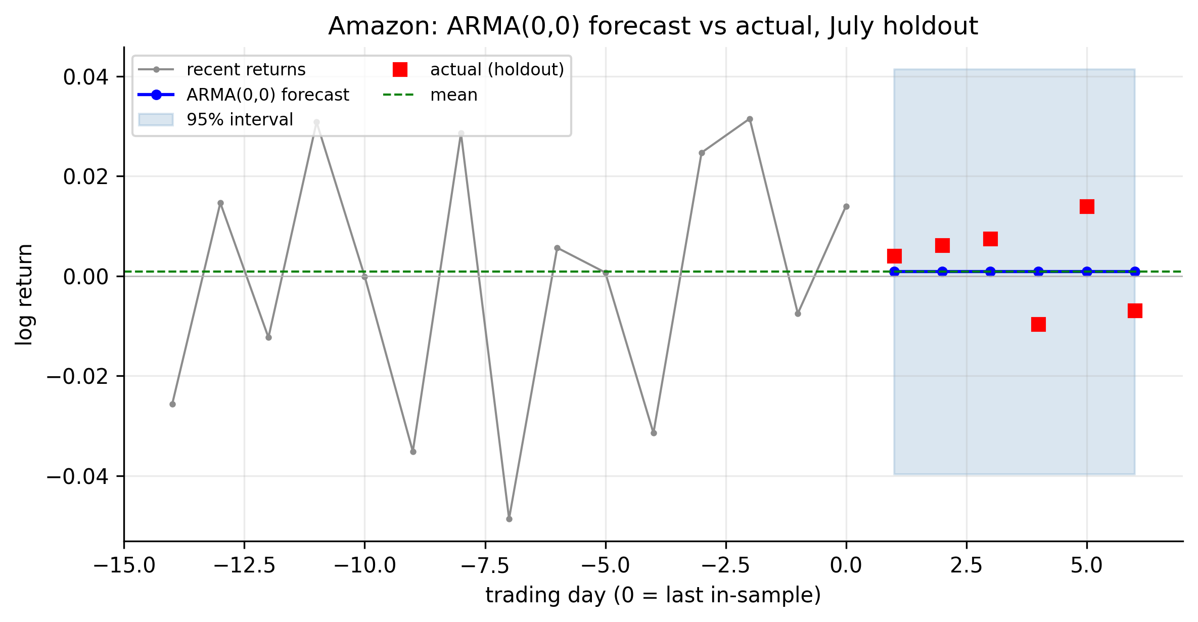
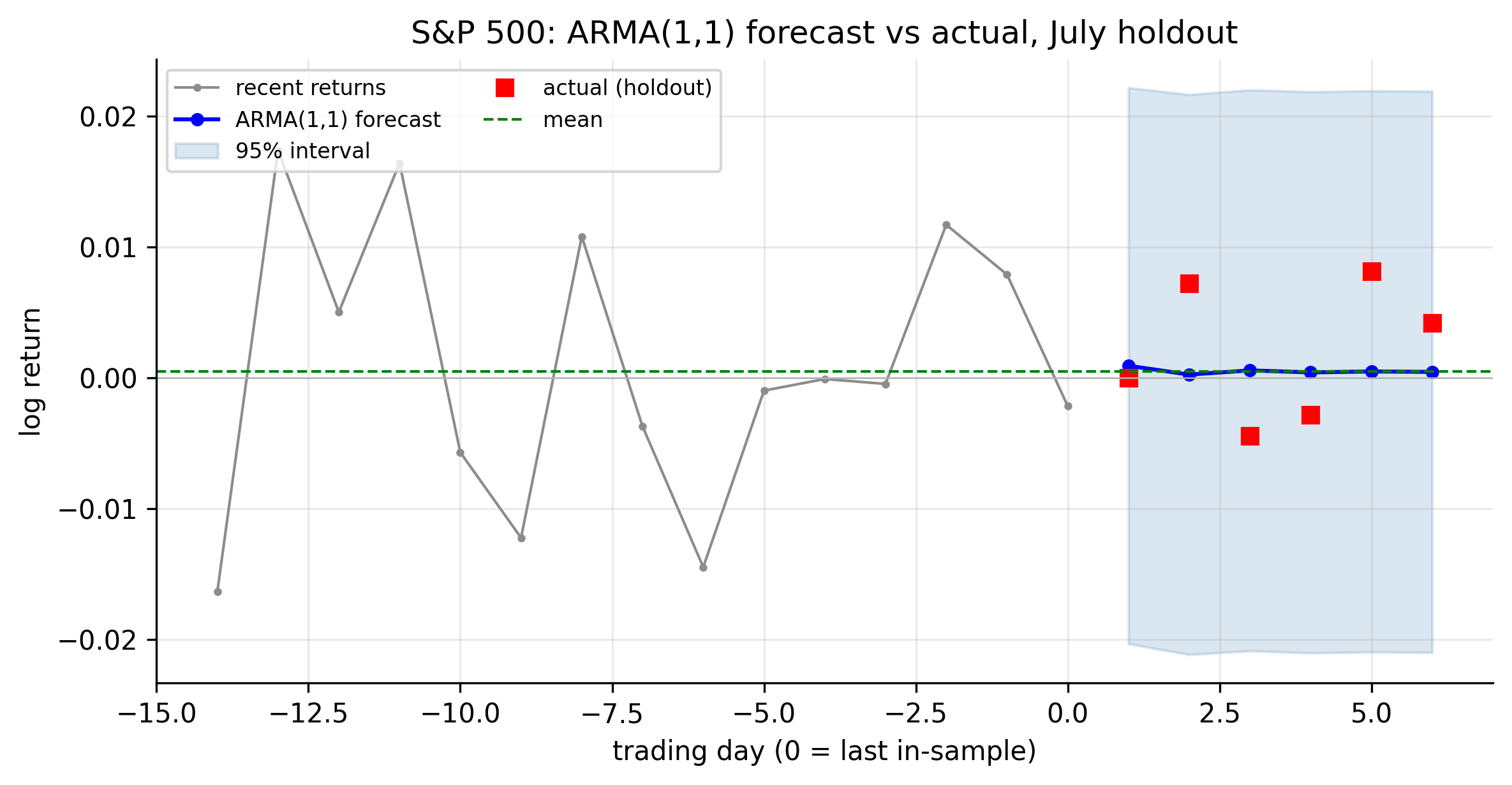
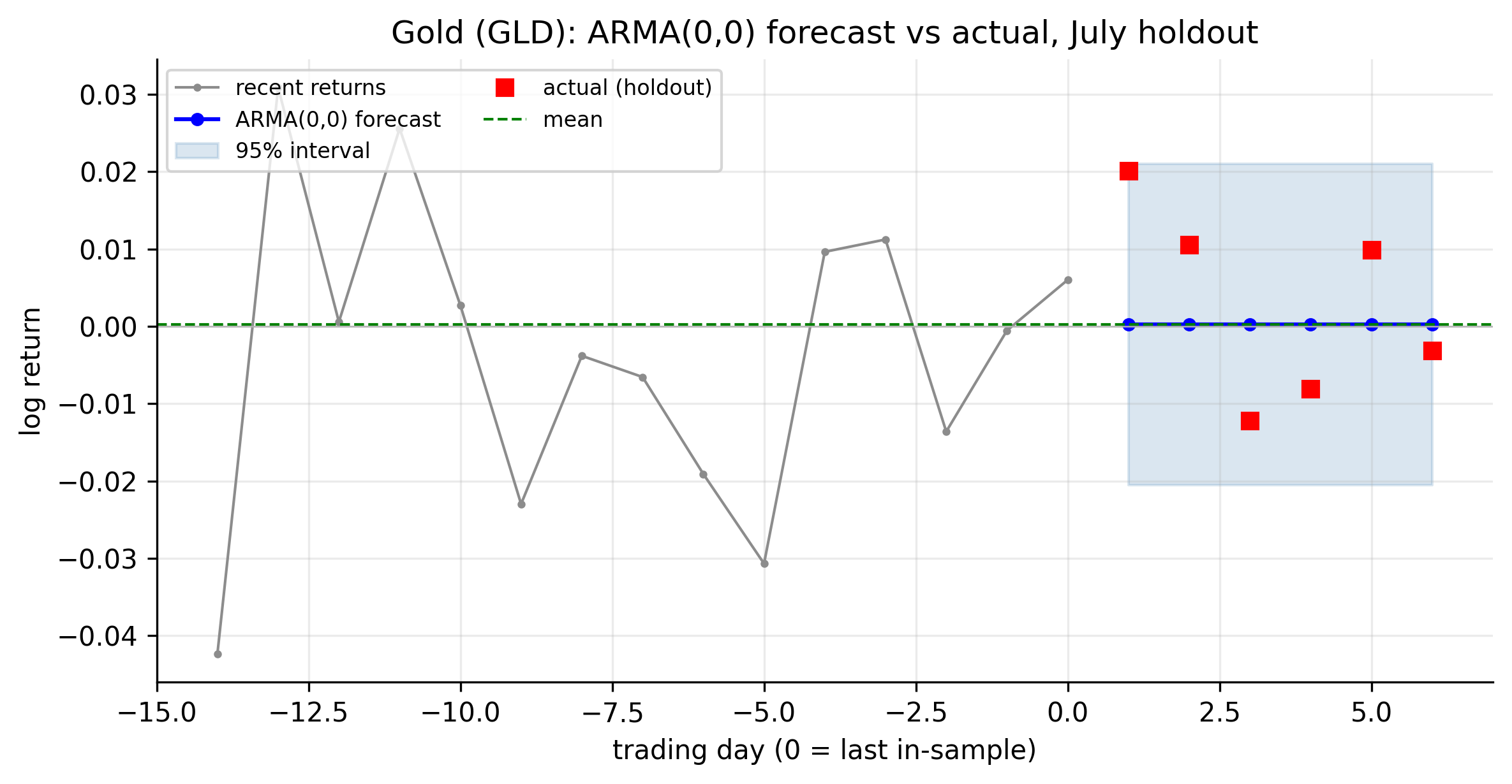
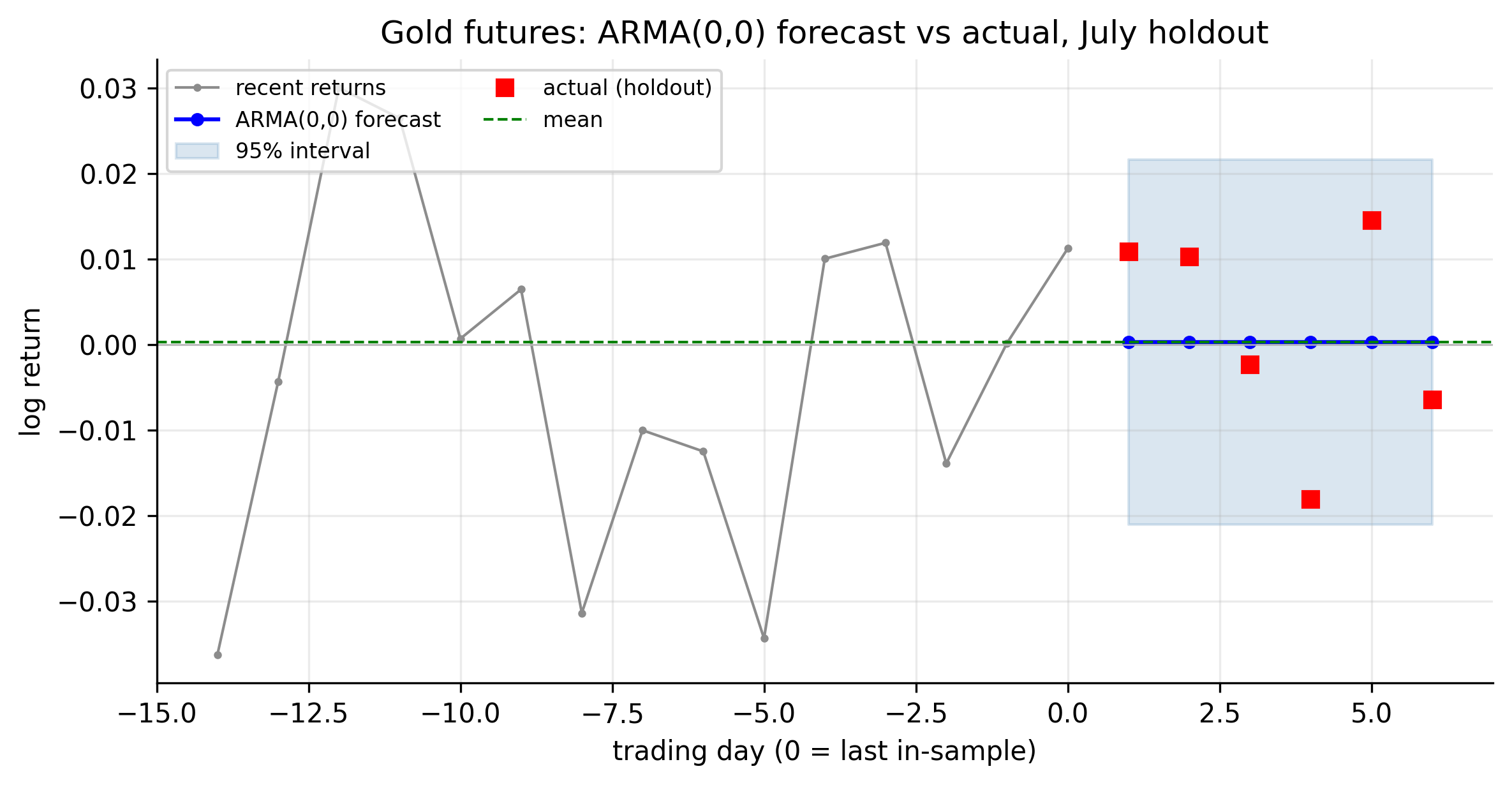
Even the S&P’s ARMA(1,1) — the most elaborate mean model in the entire analysis — produces a forecast that reverts to the mean within a few days inside an interval of about \(\pm 2\%\), with the realised returns scattered across it. The extra structure that made ARMA(1,1) the right model is real and worth capturing, but it is a one-to-two-percent refinement on an essentially unforecastable mean. The conclusion of the whole linear-modelling arc is now firm: for daily returns, the best mean model is close to the historical average, and the honest deliverable is the interval. The predictable part of these series lives in the variance — the next stage of the toolkit.
5.6 Concept check
Decide first, then expand each answer.
Q1. Why can’t you identify an ARMA(\(p,q\)) order by reading the ACF and PACF the way you do for a pure AR or MA?
- (a) ARMA models have no ACF.
- (b) For a mixed model both the ACF and the PACF tail off — neither cuts off, so there is no order to count.
- (c) The ACF and PACF are identical for ARMA.
- (d) ARMA models are never stationary.
(b). AR cuts off in the PACF, MA in the ACF; a mix cuts off in neither. That is why we use the EACF or an information-criterion grid search instead.
Q2. An ARMA(\(p,q\)) model is stationary provided:
- (a) the MA polynomial’s roots are outside the unit circle.
- (b) the AR polynomial’s roots are outside the unit circle.
- (c) \(p = q\).
- (d) all coefficients are positive.
(b). Stationarity is an AR-part property (roots of \(1-\phi_1z-\cdots\) outside the unit circle). The MA-part roots govern invertibility, a separate condition.
Q3. A fitted ARMA(1,1) returns \(\hat\phi_1 = 0.60\) and \(\hat\theta_1 = -0.59\). What should you suspect?
- (a) A strong, genuine ARMA signal.
- (b) Parameter redundancy — the AR and MA factors nearly cancel, so the series is effectively white noise and the model is over-parameterised.
- (c) The series has a unit root.
- (d) Nothing; the fit is fine.
(b). With \(\phi_1 \approx -\theta_1\) the common factors nearly cancel, leaving a near-white-noise process fitted by two large, unstable, offsetting coefficients. Prefer the simpler model. (Our S&P fit, \(\phi_1=-0.475\), \(\theta_1=+0.355\), does not cancel, so it is legitimate.)
Q4. For the S&P 500, ARMA(1,1) and AR(8) achieve almost the same fit (\(R^2 \approx 0.018\)). Why prefer the ARMA(1,1)?
- (a) It fits much better.
- (b) Parsimony — it captures the same structure with two parameters instead of eight, so it generalises better and BIC prefers it.
- (c) AR models are never valid for indices.
- (d) It has a higher \(R^2\).
(b). Same fit, far fewer parameters. The S&P’s sign-changing ACF needs many AR lags but only one AR + one MA term, and BIC rewards the parsimonious model.
Q5. In an ARMA(1,1) forecast, the moving-average term \(\theta_1 a_t\) affects:
- (a) every forecast horizon equally.
- (b) only the one-step-ahead forecast; from two steps out the forecast follows pure AR(1) reversion to the mean.
- (c) nothing — MA terms don’t affect forecasts.
- (d) only horizons beyond \(q\).
(b). The MA memory lasts \(q=1\) step, so the last shock enters only the one-step forecast; thereafter the AR part carries the forecast geometrically back to \(\mu\).
- ARMA(\(p,q\)) (Equation 5.1) combines AR and MA terms; it is stationary via the AR roots and invertible via the MA roots, with mean \(\phi_0/(1-\sum\phi_i)\).
- Its ACF and PACF both tail off (Table 5.1), so order is chosen by the EACF or an information-criterion grid, not by reading a cutoff.
- On our data, four series are white noise, Microsoft is a single lag, and the S&P 500 is a genuine ARMA(1,1) — capturing with two parameters what AR needed eight for (Table 5.2). That parsimony is the point of ARMA.
- Beware parameter redundancy (\(\phi_1 \approx -\theta_1\)): near-cancelling factors signal an over-fit model.
- Even the best ARMA mean forecast reverts to the mean inside a wide interval; the linear-modelling arc ends where it began — the mean of daily returns is barely forecastable, and the predictability lives in the variance, next.