4 Moving-Average Models
The AR model of Section 3.5 builds the mean from the series’ own past values. The moving-average (MA) model builds it instead from the past shocks — the white-noise innovations that hit the series. It is the natural counterpart to the AR model, and it comes with a lesson that our data will make vivid: for a series whose only serial correlation is a single lag, the AR and MA descriptions are nearly interchangeable. We follow the same path as before — definition, properties, identification, goodness of fit, forecasting — and apply each step to the six tickers.
The R code uses stats/forecast; Python uses statsmodels.
4.1 Simple MA models
A moving-average (MA) model builds today’s value from the current and most recent random shocks, rather than from past values.
A moving-average model of order \(q\), MA(\(q\)), expresses today’s return as a weighted average of the current and most recent \(q\) shocks:
\[ r_t = \mu + a_t + \theta_1 a_{t-1} + \theta_2 a_{t-2} + \cdots + \theta_q a_{t-q}, \tag{4.1}\]
with \(\{a_t\}\) white noise. The name is literal: \(r_t\) is a moving average of the innovation stream. It is the special case of the linear (Wold) representation Equation 3.5 in which only finitely many weights are nonzero — \(\psi_0 = 1\), \(\psi_i = \theta_i\) for \(i \le q\), and \(\psi_i = 0\) afterward. The MA(1), \(r_t = \mu + a_t + \theta_1 a_{t-1}\), is the workhorse: today’s return is this period’s shock plus a fraction of last period’s.
4.2 Properties of MA models
MA models differ from AR models in three ways worth stating clearly.
They are always stationary. An MA(\(q\)) is a finite sum of white-noise terms, so its mean and variance are constant for any values of the \(\theta\)’s — there is no stationarity condition to check. This is the opposite of the AR case, where \(|\phi|<1\) (roots outside the unit circle) was required. Concretely,
\[ E[r_t] = \mu, \qquad \operatorname{Var}(r_t) = \sigma^2\bigl(1 + \theta_1^2 + \cdots + \theta_q^2\bigr). \tag{4.2}\]
Note the mean is the constant \(\mu\) — unlike the AR model, where the intercept had to be rescaled by \(1/(1-\sum\phi)\).
The ACF cuts off after lag \(q\). This is the identification signature. Because \(r_t\) and \(r_{t-k}\) share no common shocks once \(k > q\), their correlation is exactly zero beyond lag \(q\). For the MA(1),
\[ \rho_1 = \frac{\theta_1}{1 + \theta_1^2}, \qquad \rho_k = 0 \;\text{ for } k \ge 2, \tag{4.3}\]
while the PACF tails off gradually. This is the exact mirror image of the AR model (Table 3.2), whose PACF cuts off and ACF tails off.
Invertibility. Different \(\theta\) values can produce the same ACF (for MA(1), \(\theta_1\) and \(1/\theta_1\) give identical \(\rho_1\)). To make the model unique — and to let it be rewritten as an infinite-order AR — we require the roots of \(1 + \theta_1 z + \cdots + \theta_q z^q = 0\) to lie outside the unit circle (for the MA(1), \(|\theta_1| < 1\)). We always report the invertible solution.
4.3 Identifying MA models
Identification mirrors the AR procedure with the roles of the ACF and PACF swapped: the ACF now supplies the order (it cuts off after lag \(q\)), and an information criterion confirms it. Looking back at the ACF grid in Figure 3.1, our returns’ autocorrelations are essentially zero beyond lag 1, and lag 1 itself is significant only for Microsoft and the S&P 500 (marginally Apple). So the ACF points to an MA(1) for Microsoft and the S&P and MA(0) — white noise — for the rest, exactly mirroring the AR verdict. AIC/BIC agree:
est_return <- function(sym) {
  d <- read.csv(sprintf("data/%s.csv", sym)); d$Date <- as.Date(d$Date)
  diff(log(d$Adjusted[d$Date <= as.Date("2026-07-01")]))
}
# MA order by BIC (fit q = 0,1,2 and compare)
for (s in c("AAPL","MSFT","AMZN","SPX","GLD","GCF")) {
  r   <- est_return(s)
  bic <- sapply(0:2, function(q) BIC(arima(r, order = c(0, 0, q), method = "ML")))
  cat(s, " MA-order (BIC):", which.min(bic) - 1, "\n")
}
arima(est_return("SPX"), order = c(0, 0, 1))     # SPX MA(1): estimate theta
import pandas as pd, numpy as np
from statsmodels.tsa.arima.model import ARIMA
def est_return(sym):
d = pd.read_csv(f"data/{sym}.csv", parse_dates=["Date"]).set_index("Date")
return np.log(d[d.index <= "2026-07-01"]["Adjusted"]).diff().dropna()
for s in ["AAPL","MSFT","AMZN","SPX","GLD","GCF"]:
bic = [ARIMA(est_return(s), order=(0, 0, q)).fit().bic for q in range(3)]
print(s, "MA-order (BIC):", int(np.argmin(bic)))| Ticker | \(\hat\rho_1\) | MA order (BIC) | \(\hat\theta_1\) | AR order (BIC) |
|---|---|---|---|---|
| AAPL | −0.038 | 0 | — | 0 |
| MSFT | −0.097 | 1 | −0.10 | 1 |
| AMZN | −0.016 | 0 | — | 0 |
| SPX | −0.119 | 1 | −0.11 | 8 |
| GLD | −0.003 | 0 | — | 0 |
| GCF | −0.032 | 0 | — | 0 |
4.3.1 AR(1) and MA(1) are nearly the same model here
Table 4.1 contains the chapter’s key insight. For a series whose only serial correlation is a single small \(\rho_1\), both descriptions fit it: the AR(1) produces one PACF spike, the MA(1) produces one ACF spike, and with correlation only at lag 1 those are the same spike. The data cannot tell the two models apart. Fitting both to Microsoft and the S&P makes the point numerically:
| Series | AR(1) \(\hat\phi_1\) | AR(1) resid. SD | MA(1) \(\hat\theta_1\) | MA(1) resid. SD |
|---|---|---|---|---|
| MSFT | −0.097 | 1.6453% | −0.100 | 1.6449% |
| SPX | −0.119 | 1.0858% | −0.110 | 1.0866% |
The estimated coefficients nearly coincide (\(\hat\theta_1 \approx \hat\phi_1 \approx \hat\rho_1\)) and the residual standard deviations match to four decimal places. The reason is visible in the algebra: for a small parameter, the MA(1) autocorrelation \(\rho_1 = \theta_1/(1+\theta_1^2) \approx \theta_1\), while the AR(1) has \(\rho_1 = \phi_1\) — so both parameters just equal the lone lag-1 correlation. For these series the choice between AR(1) and MA(1) is immaterial. The distinction only bites when a series has richer structure — which points to the one asymmetry in Table 4.1: the S&P’s AR order was \(8\) but its MA order is \(1\). The S&P’s ACF is (weakly) significant at lag 2 as well as lag 1, so neither a low-order AR nor a low-order MA fully captures it; a mixed ARMA model, next, does the job more parsimoniously.
At the monthly frequency the story collapses entirely: as we saw for AR (Table 3.5), every series is white noise, so the MA order is \(0\) for all six. Aggregation erases what little short-horizon structure the daily data held.
4.4 Goodness of fit
The diagnostics are the same as for AR, with the same sobering conclusion. A fitted MA model should leave white-noise residuals (Ljung–Box on \(\hat a_t\) should not reject), and its explanatory power is tiny: because the MA(1) and AR(1) residual variances coincide (Table 4.2), Microsoft’s MA(1) explains about \(1\%\) of return variance, the S&P’s about \(1.4\%\). And exactly as before, whitening the linear dependence leaves the squared-residual correlation of Figure 3.3 untouched — the volatility clustering is still there, still waiting for GARCH.
fit <- arima(est_return("SPX"), order = c(0, 0, 1))       # MA(1)
Box.test(residuals(fit), lag = 10, type = "Ljung-Box")    # residuals white noise?
1 - fit$sigma2 / var(est_return("SPX"))                   # approx R^2
from statsmodels.stats.diagnostic import acorr_ljungbox
fit = ARIMA(est_return("SPX"), order=(0, 0, 1)).fit()
print(acorr_ljungbox(fit.resid, lags=[10]))
print(1 - fit.resid.var() / est_return("SPX").var())4.5 Forecasting
MA forecasting has a defining feature: finite memory. An MA(\(q\)) remembers only the last \(q\) shocks, so its forecast reverts to the mean abruptly once the horizon passes \(q\):
\[ \hat r_t(h) = \begin{cases} \mu + \sum_{j=h}^{q} \theta_j\, a_{t+h-j}, & h \le q,\\[4pt] \mu, & h > q. \end{cases} \tag{4.4}\]
For an MA(1) this means the one-step forecast is \(\mu + \theta_1 a_t\) — a single adjustment based on the last observed shock — and every forecast from two steps out is exactly the mean. The forecast-error variance jumps from \(\sigma^2\) at \(h=1\) to the full unconditional variance \(\sigma^2(1+\theta_1^2)\) for \(h \ge 2\) and stays there. This is a sharp contrast with the AR(1), whose forecast decays to the mean gradually (as \(\phi_1^h\)); the MA(1) snaps to it after one step.
The carousel below runs the MA forecast across all six tickers over the July holdout. Step through with the arrows or dots.
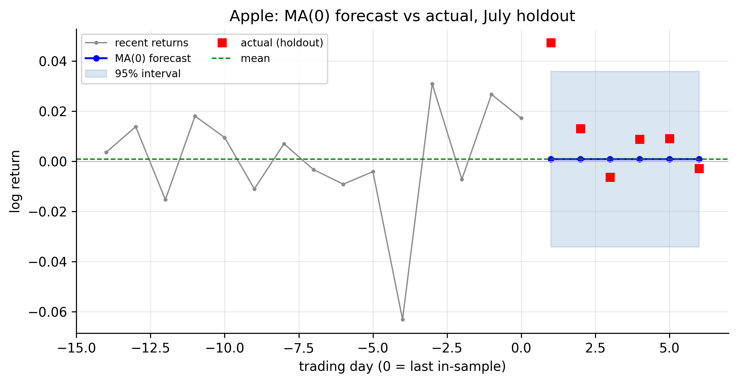
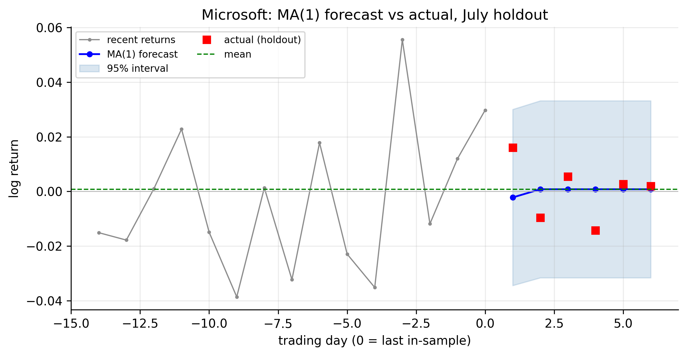
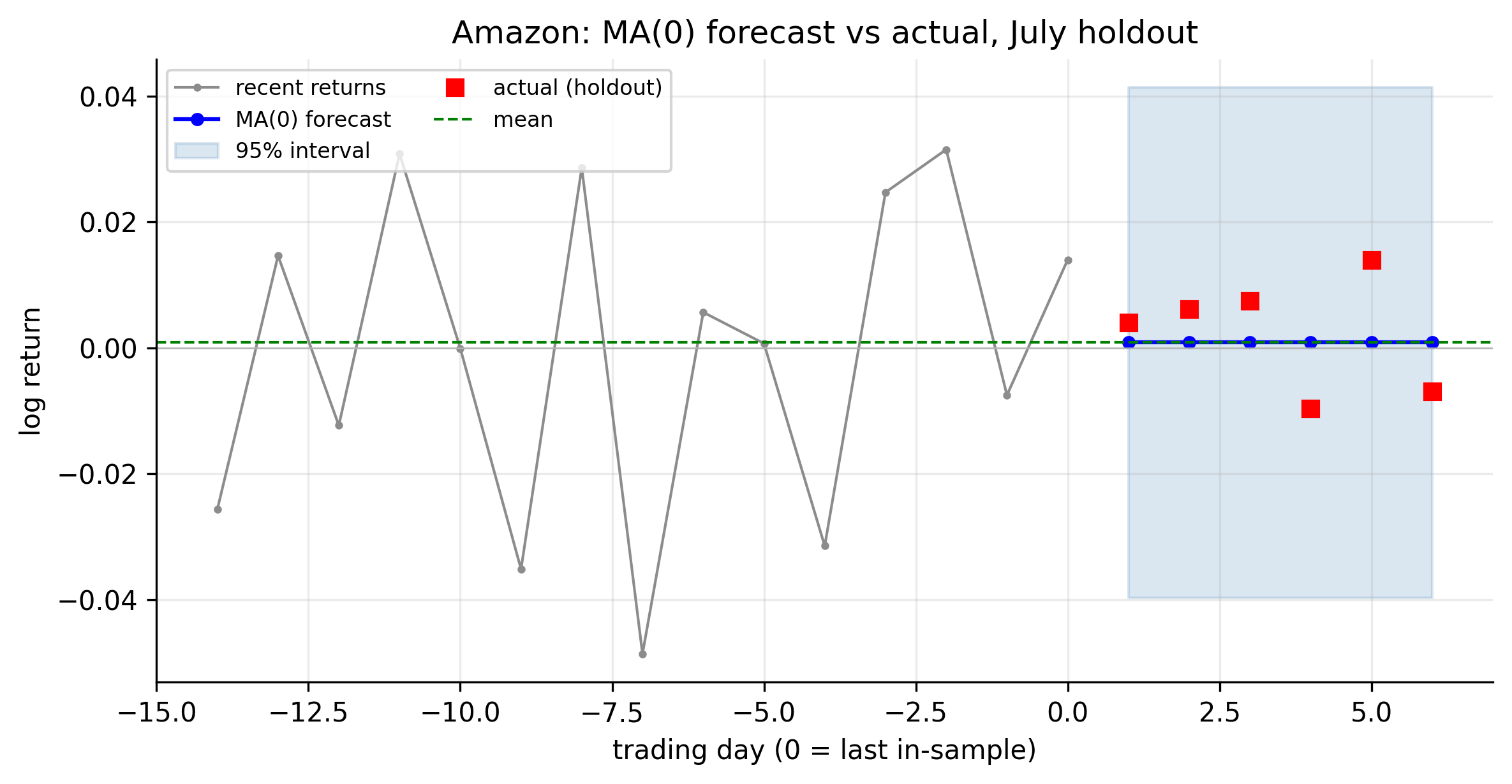
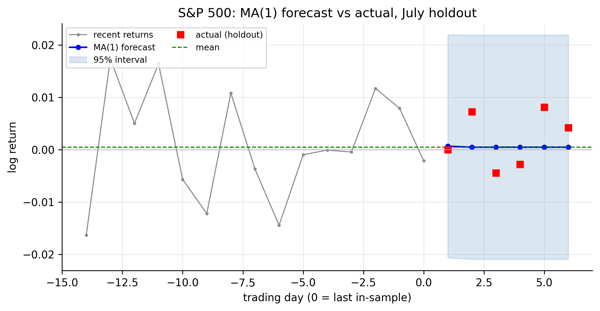
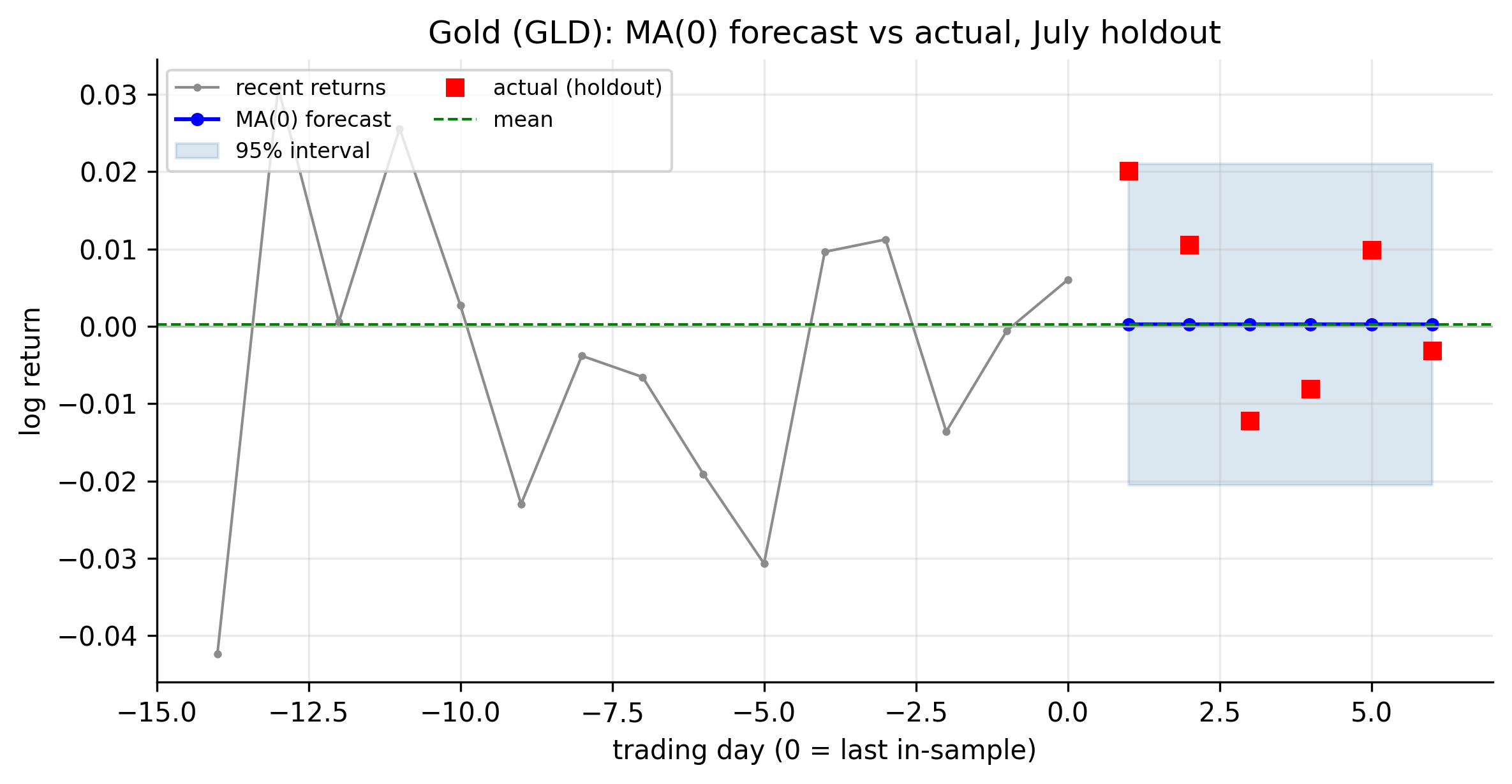
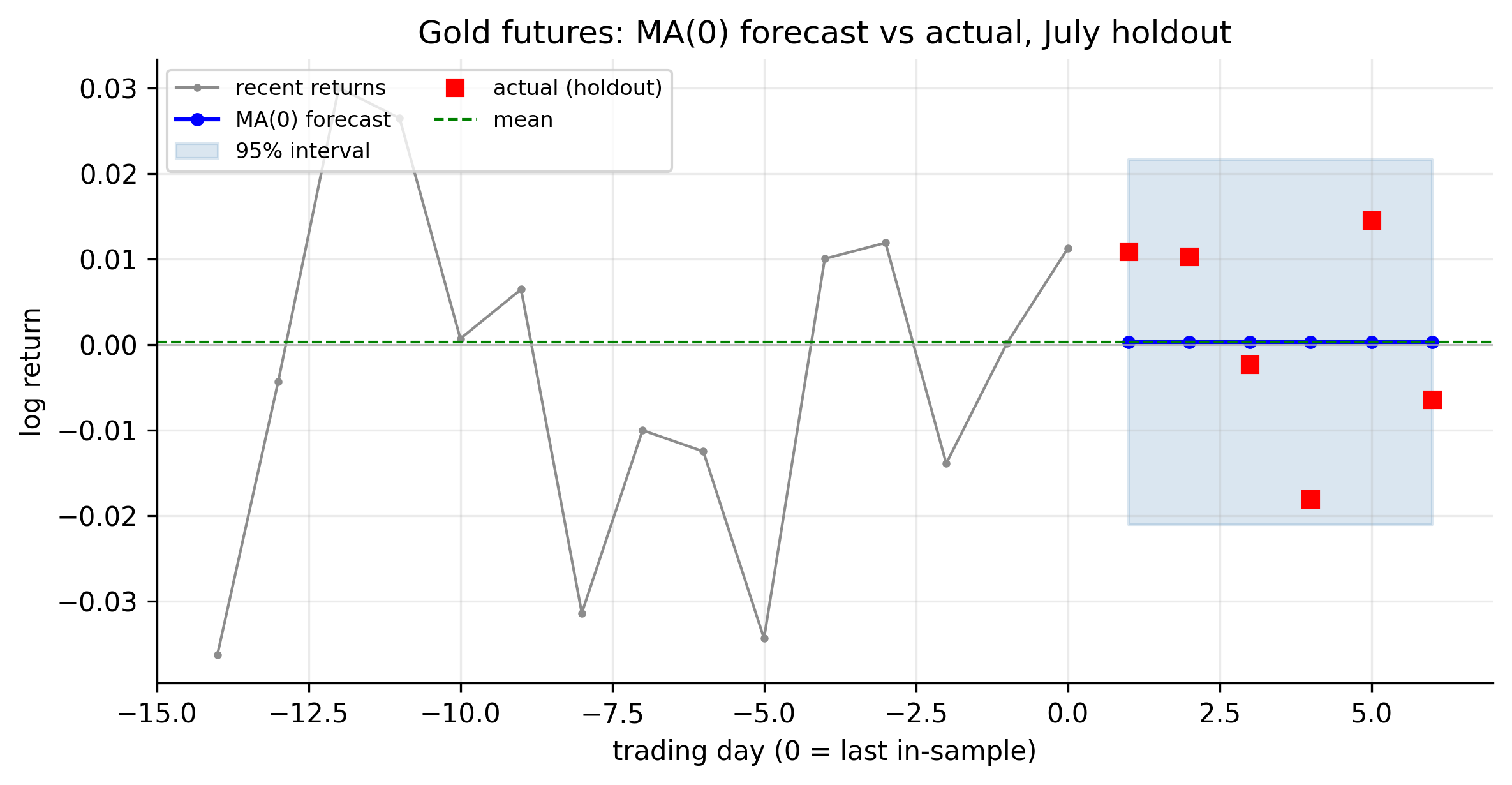
The panels tell the by-now-familiar story, with one MA-specific twist. The four MA(0) series (Apple, Amazon, both gold) forecast a flat line at the mean from day one. Microsoft and the S&P — the MA(1) fits — show a single one-step blip (the \(\theta_1 a_t\) term: for Microsoft it dips to \(-0.22\%\), pulled down because the last shock was positive and \(\theta_1<0\)) and then snap exactly to the mean at day two, where an AR(1) would have eased toward it. Either way the verdict is unchanged: the interval dwarfs the point forecast, the realised returns scatter across it, and the mean of daily returns stays unforecastable.
4.6 Concept check
Decide first, then expand each answer.
Q1. Which condition must an MA(\(q\)) model satisfy to be stationary?
- (a) The roots of its characteristic polynomial must lie outside the unit circle.
- (b) \(|\theta_1| < 1\).
- (c) None — a finite MA is always stationary.
- (d) Its mean must be zero.
(c). An MA(\(q\)) is a finite sum of white-noise terms, so its mean and variance are constant for any \(\theta\)’s. (The \(|\theta|<1\) condition is invertibility, not stationarity — a different requirement.)
Q2. A series has an ACF that is significant at lag 1 and essentially zero afterward, with a PACF that decays gradually. This is the signature of:
- (a) an AR(1).
- (b) an MA(1).
- (c) white noise.
- (d) a random walk.
(b). MA(\(q\)): ACF cuts off after lag \(q\), PACF tails off. A single ACF spike with a decaying PACF is MA(1) — the mirror image of the AR(1) signature.
Q3. We fit both an AR(1) and an MA(1) to the S&P 500 and get virtually identical residuals (\(\hat\phi_1 \approx \hat\theta_1 \approx -0.11\)). Why?
- (a) A coding error.
- (b) With correlation only at lag 1, both models capture the same single autocorrelation, so they are observationally near-equivalent.
- (c) AR and MA models are always identical.
- (d) The S&P is a random walk.
(b). For a small lag-1 correlation, \(\rho_1 = \theta_1/(1+\theta_1^2) \approx \theta_1\) (MA) and \(\rho_1 = \phi_1\) (AR), so both parameters equal the lone lag-1 correlation. The choice is immaterial here; the models diverge only with richer structure.
Q4. In an MA(1) model \(r_t = \mu + a_t + \theta_1 a_{t-1}\), the unconditional mean of \(r_t\) is:
- (a) \(\mu/(1-\theta_1)\).
- (b) \(\mu\).
- (c) \(\theta_1\).
- (d) zero.
(b). Since \(E[a_t]=0\), the mean is just the constant \(\mu\). (Contrast the AR(1), whose mean is \(\phi_0/(1-\phi_1)\) — the intercept is not the mean there.)
Q5. For an MA(1) with \(\theta_1 = -0.10\), the forecast three steps ahead equals:
- (a) \(\mu + \theta_1^3(r_t - \mu)\).
- (b) the last observed value.
- (c) exactly the mean \(\mu\).
- (d) zero.
(c). An MA(1) has one-period memory: only the one-step forecast uses the last shock (\(\mu + \theta_1 a_t\)); every forecast from two steps out is exactly \(\mu\). Answer (a) is the AR(1) forecast, which reverts gradually instead.
- An MA(\(q\)) (Equation 4.1) builds the return from the last \(q\) shocks; it is always stationary, and its mean is simply the constant \(\mu\) (Equation 4.2).
- Its ACF cuts off after lag \(q\) while the PACF tails off — the mirror image of the AR model, and the tool for identifying the order.
- On our data the MA order matches the AR order (MA(1) for Microsoft and the S&P, MA(0) for the rest), and for a single lag-1 correlation AR(1) and MA(1) are observationally near-equivalent (Table 4.2).
- MA forecasts have finite memory: they revert to the mean exactly after \(q\) steps, and — like the AR forecasts — carry so little signal that the interval is the real deliverable.
- The S&P’s mismatch (AR order 8 vs MA order 1) flags structure that neither pure model captures parsimoniously — the motivation for ARMA next.